The most fundamental idea we will need is the continuum hypothesis.  In simple terms this says that when dealing with fluids we can ignore the fact that they actually consist of billions of individual  molecules (or atoms) in a rather small region, and instead treat the properties of that region as if it were a continuum.  By appealing to this assumption we may treat any fluid property as varying continuously from one point to the next within the fluid; this  clearly  would not be possible without  this  hypothesis.  To understand  how physical quantities are defined in the continuum model we consider the following experiment to observe hob density of fluid is related to its molecular  structure. At time t we consider a cube with the width α occupied by fluid centered at x0 .The average density of the fluid is  ρα=Mα/α3 , where Mα  is the mass of the fluid inside of the cube.  To define the density ρ(x0 , t) it is examined  what happens  as α approaches  zero.  The  graph  fig.  4) shows the results.  In region II, since there are many particles inside the cube, the average density ρα vary  very little.  If, however α were on the order of molecular distances, ∼ 10e−9  meters, the may be only a few molecules in the cube and one will observe large fluctuations in ρα. Such rapid  fluctuations are depicted in region I, It seems unreasonable therefore to define ρ(x0 , t) as the limiting value of ρα as α → 0. Rather ρ(x0 , t) should be defined as

where α∗ is the value of α where density begin to vary violently, here for example α∗ = 10e−9 meters.  In a similar fashion other physical quantities can be considered as point functions in continuously distributed matter without regard  to its molecular  or atomic structure.

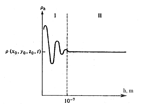
Fig. 4: Graph of the average density ρα versus the with α.