Basic Concepts

To understand the fairly advanced statistics underlying quality control, a certain basic level of statistics is assumed by most texts dealing with this subject. The brief introduction given below should help to lead readers into the various texts dealing with quality control.

The arithmetic mean, or mean, is the average value of a set of data. Its value can be found by adding together the values of the members of the set and then dividing by the number of members in the set. Mathematically:

X=(X₁+X₂+….+X_N)/N

Thus the mean of the set of numbers 4, 6, 9, 3 and 8 is (4+6+9+3+8)/5=6.

The median is either the middle value or the mean of the two middle values of a set of numbers arranged in order of magnitude. Thus the numbers 3, 4, 5, 6, 8, 9, 13 and 15 have a median value of (6+8)/2=7, and the numbers 4, 5, 7, 9, 10, 11, 15, 17 and 19 have a median value of 10.

The mode is the value in a set of numbers which occurs most frequently. Thus the set 2, 3, 3, 4, 5, 6, 6, 6, 7, 8, 9 and 9 has a modal value of 6.

The range of a set of numbers is the difference between the largest value and the smallest value. Thus the range of the set of numbers 3, 2, 9, 7, 4, 1, 12, 3, 17 and 4 is 17-1=16.

The standard deviation, sometimes called the root mean square deviation, is defined by:

s=√[(X₁-X)²+(X₂-X)²+…+(X_N-X)²]/N

Thus for the numbers 2, 5 and 11, the mean in (2+5+11)/3, that is 6. The standard deviation is:

s=√[(2-6)²+(5-6)²+(11-6)²]/3

=√(16+1+25)/3

=√14

≈3.74

Usually s is used to denote the standard deviation of a population (the whole set of values) and σ is used to denote the standard deviation of a sample.

Probability

When an event can happen x ways out of a total of n possible and equally likely ways, the probability of the occurrence of the event is given by p= x/n. The probability of an event occurring is therefore a number between 0 and 1. If q is the probability of an event not occurring it also follows that p+q=1. Thus when a fair six-sided dice is thrown, the probability of getting a particular number, say a three, is 1/6, since there are six sides and the number three only appears on one of the six sides.

Binomial distribution

The binomial distribution as applied to quality control may be stated as follows.

The probability of having 0, 1, 2, 3, …, n defective items in a sample of n items drawn at random from a large population, whose probability of a defective item is p and of a non-defective item is q, is given by the successive terms of the expansion of (q+p)ⁿ, taking terms in succession from the right.

Thus if a sample of, say, four items is drawn at random from a machine producing an average of 5% defective items, the probability of having 0, 1, 2, 3 or 4 defective items in the sample can be determined as follows. By repeated multiplication:

(q+p)⁴=q⁴+4q³p+6q²p²+4qp³+p⁴

Then the values of q and p are q=0.95 and p=0.05. Thus

(0.95+0.05)⁴=0.95⁴+(4×0.95³×0.05)+(6×0.95²×0.05²)+(4×0.95+0.05³)+0.05⁴

=0.8145+0.1715+0.011354+…….

This indicates that

(a) 81% of the samples taken are likely to have no defective items in them.

(b) 17% of the samples taken are likely to have one defective item.

(c) 1% of the samples taken are likely to have two defective items.

(d) There will hardly ever be three or four defective items in a sample.

As far as quality control is concerned, if by repeated sampling these percentages are roughly maintained, the inspector is satisfied that the machine is continuing to produce about 5% defective items. However, if the percentages alter then it is likely that the defect rate has also altered. Similarly, a customer receiving a large batch of items can, by random sampling, find the number of defective items in the samples and by using the binomial distribution can predict the probable number of defective items in the whole batch.

Poisson distribution

The calculations involved in a binomial distribution can be very long when the sample number n is larger than about six or seven, and an approximation to them can be obtained by using a Poisson distribution. A statement for this is:

When the chance of an event occurring at any instant is constant and the expectation np of the event occurring is λ, then the probabilities of the event occurring 0, 1, 2, 3, 4, … times are given by:

e^-λ, λe^-λ, λ²e^-λ/2!, λ³e^-λ/3!, λ⁴e^-λ/4!,……

where:

e is the constant 2.718 28 … and 2!=2×1,3!=3×2×1,4!=4×3×2×1, and so on (where 4! is read ‘four factorial’).

Applying the Poisson distribution statement to the machine producing 5% defective items, used above to illustrate a use of the binomial distribution, gives:

expectation np=4×0.05=2

probability of no defective items is e^–λ=e^-0.2=0.8187

probability of one defective items is λe^-λ=0.2e^-0.2=0.1637

probability of two defective items is λ²e^-λ/2!=0.2²e^-0.2/2=0.0164

It can be seen that these probabilities of approximately 82%, 16% and 2% compare quite well with the results obtained previously.

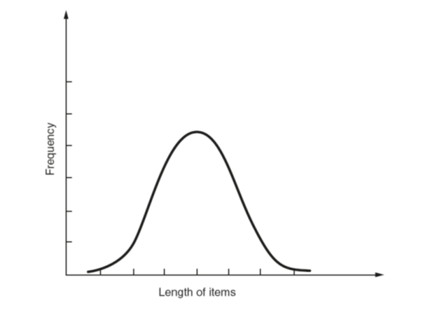
Normal distribution

Data associated with measured quantities such as mass, length, time and temperature is called continuous, that is, the data can have any values between certain limits. Suppose that the lengths of items produced by a certain machine tool were plotted as a graph, as shown in the figure; then it is likely that the resulting shape would be mathematically definable. The shape is given by y= (1/σ)e^z, where z=-x²/2σ², σ is the standard deviation of the data, and x is the frequency with which the data occurs. Such a curve is called a normal probability or a normal distribution curve.

Important properties of this curve to quality control are:

 

• The area enclosed by the curve and vertical lines at +1 standard deviation from the mean value is approximately 67% of the total area.

(b) The area enclosed by the curve and vertical lines at +2 standard deviations from the mean value is approximately 95% of the total area.

(c) The area enclosed by the curve and vertical lines at +3 standard deviations from the mean value is approximately 99.75% of the total area.

(d) The area enclosed by the curve is proportional to the frequency of the population.

To illustrate a use of these properties, consider a sample of 30 round items drawn at random from a batch of 1000 items produced by a machine. By measurement it is established that the mean diameter of the samples is 0.503 cm and that the standard deviation of the samples is 0.0005 cm. The normal distribution curve theory may be used to predict the reject rate if, say, only items having a diameter of 0.502–0.504 cm are acceptable. The range of items accepted is 0.504-0.502=0.002 cm. Since the standard deviation is 0.0005 cm, this range corresponds to +2 standard deviations. From (b) above, it follows that 95% of the items are acceptable, that is, that the sample is likely to have 28 to 29 acceptable items and the batch is likely to have 95% of 1000, that is, 950 acceptable items.

This example was selected to give exactly +2 standard deviations. However, sets of tables are available of partial areas under the standard normal curve, which enable any standard deviation to be related to the area under the curve.